What is the k-Value?

The modulus of subgrade reaction — commonly called the k-value after a spring constant being called k in physics — quantifies how stiff the ground is beneath a concrete slab. It is defined as the ratio of applied pressure to the resulting surface deflection:

A higher k-value means a stiffer subgrade that deflects less under load. A lower k-value means a softer subgrade that deflects more, putting greater bending stress into the concrete above it. In slab-on-ground design, k-value impacts the slab thickness required to carry a given set of loads within allowable stress limits.

Importantly, k-value is not a fundamental soil property — it depends on the plate size used to measure it, the rate at which load is applied, the moisture state of the soil, and the stiffness of deeper layers. It must be interpreted carefully depending on how it was obtained and which design procedure will use it.

The Two Foundation Models

Two idealized models dominate foundation analysis for concrete slabs, each capturing a different extreme of real soil behavior.

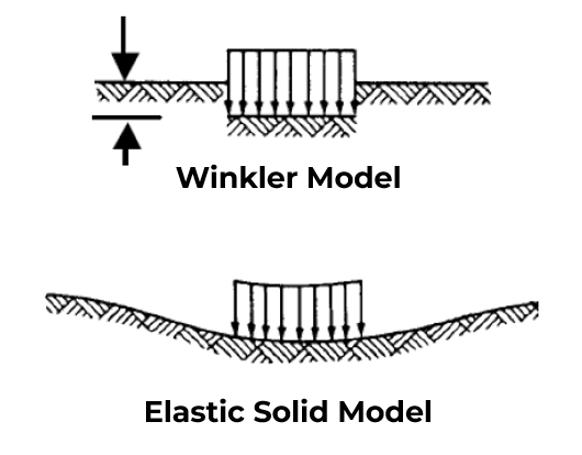
The Winkler model (dense liquid model) represents the soil as a bed of independent springs, each with a linear spring constant equal to k. Deflection occurs only where load is applied — there is no shear transfer between adjacent spring elements. This makes it simple and computationally efficient; it is used in Westergaard’s analytical solutions and in finite element programs such as ISLAB2000. Its main weakness is that it underestimates the true supporting area of real soil because actual shear resistance spreads load beyond the loaded footprint.

The Elastic Solid model treats the subgrade as a continuous elastic half-space. Load at any point causes deflections throughout the entire soil mass, capturing the shear coupling that the Winkler model ignores. However, by modeling discrete soil particles as a solid continuum, it overestimates cohesion and friction. Its use is typically limited to finite element analysis with advanced constitutive soil models.

Neither model is a true representation of real soil behavior. The AASHTOWare Pavement ME and this calculator both use an approach that lies between the two extremes and produces more realistic results for layered support systems.

Static, Dynamic, and Effective Dynamic k-Value

Not all k-values are the same. Three distinct definitions appear in practice, and confusing them may lead to design errors.

The static k-value is determined by the ASTM D1196 plate load test: a rigid steel plate is loaded incrementally on the prepared subgrade surface and the resulting settlements are recorded. By convention, k is taken at a deflection of 0.05 in (1.27 mm). This test reflects the stiffness of the soil within roughly twice the plate diameter and is the traditional basis for concrete pavement and slab-on-ground design. It is expensive and time-consuming, so it not routinely done in practice.

The dynamic k-value is obtained by back-calculation from the Falling Weight Deflectometer (FWD): a standard 9-kip (40 kN) impulse load is dropped and the resulting deflection bowl is measured, then k is back-calculated. FWD-derived dynamic k-values are consistently found to be approximately twice the static k-value on the same subgrade, because pore water pressures do not have time to dissipate under the brief dynamic load.

The effective dynamic k-value, as calculated in AASHTOWare Pavement ME, is not measured but computed. Surface deflections are first calculated for the multi-layer system using elastic layer theory under a simulated 9-kip (40 kN) FWD load, and a k-value is then back-calculated from those computed deflections. This makes it a derived intermediate quantity that requires adjustment before use as a design input. A similar approach is taken in this calculator.

Why a New Method Was Needed

For most of concrete flatwork’s history, engineers either measured k directly with plate load tests or estimated it from soil classification and CBR tables. As thinner concrete pavement systems demanded higher k-values and more precise subgrade characterization, the shortcomings of each existing approach became apparent.

• CBR correlation tables are fast but imprecise, valid only for single-layer conditions, and produce ranges too wide for optimized designs.
• Plate load tests give accurate static k-value directly but are expensive, slow, and cannot account for multi-layer conditions or the dynamic nature of traffic loading.
• AASHTOWare Pavement ME back-calculation is theoretically rigorous but requires combining multiple software programs (e.g., BISAR + ISLAB2000) and is too complex for routine design practice.

The Palmer-Barber multi-layer method implemented here fills this gap. It takes the subbase layer modulus and thickness as inputs, applies the Burmister elastic layer solution with a rigid-plate correction, and produces an effective dynamic k-value that balances accuracy and practical usability.

How to Use the Calculator

If only a CBR value is available, use the CBR ↔ Resilient Modulus converter at the top of the calculator page. The conversion uses the AASHTOWare Pavement ME power-law relationship, proven valid for a wide range of subgrade strengths. See the Equations page for details.

The calculator accepts as many subbase layers above the natural subgrade as you'd like. The soil is defined by its modulus and Poisson’s ratio and and is treated as a semi-infinite half-space — no thickness is entered for it. Each subbase layer is defined by its modulus and thickness.

Origins

The underlying Burmister elastic layer theory was originally developed for flexible pavement analysis and was adapted for rigid pavement subgrade characterization through the Palmer-Barber multilayer deflection solution and the Ullidtz rigid-plate pressure correction. This approach was developed by José Tomás Cañas Silva at Universidad de Los Andes (2010) under the supervision of Juan Pablo Covarrubias Vidal of TCPavements, specifically to support subgrade characterization for optimized concrete pavement design.

Validation against PCA and FAA empirical plate load test databases in Cañas Silva 2010 showed that the method’s average error is comparable to the variability between the PCA and FAA datasets themselves — meaning the method is as accurate as the empirical data it is being compared against. The Comparison page shows how results from this calculator compare to the k-value tables first developed by PCA and then propagated by ACPA.